8. Polynomial Regression from Scratch

In this assignment, first, you need to implement Polynomial Regression from Scratch using Numpy without Sklearn. After the scratch implementation, we also use the Polynomial Regression using Sklearn and compare the two models. Your main task is to improve the code from Polynomial Regression from Scratch

8.1. Introduction

Response Variable : Position

Target Variable : Salary

Equation Used : \(y = W0 * X0 + W1 * X1 + W2 * X1^{2} + .... + WN * X1^{N}\)

Why Linear?

A genuine question can be “If the equation contain powers greater than one, how come it is linear regression?” It’s a great question! Note that the powers of \(X\) are greater than one and these are actually constants. We have these values in our dataset. We care more about \(W\) and the equation combines these product of \(W\) and \(X\) linearly i.e it has the linear combination of these terms.

For Scratch Implementation:

Loss Function : Squared Error

Optimization Algorithm : SGD

Weight Initialization : Xavier Initialization

8.2. Polynomial Regression from Scratch without SKlearn

8.2.1. Importing the Dependencies

#importing the required packages
import numpy as np
import pandas as pd
import matplotlib.pyplot as plt

8.2.2. Get the Data and Data Preprocessing

#Get the dataset
dataset = pd.read_csv(r'../../dataset/Position_Salaries.csv')

#Get a glimpse of the Dataset
dataset.head()

	Position	Level	Salary
0	Business Analyst	1	45000
1	Junior Consultant	2	50000
2	Senior Consultant	3	60000
3	Manager	4	80000
4	Country Manager	5	110000

#Separating the independent and dependent features
#Dependent feature
y = np.asarray(dataset['Salary'].values.tolist()) 

# Independent Feature
X = np.asarray(dataset['Level'].values.tolist())

# Reshaping the independent feature
X = X.reshape(-1,1)
X

array([[ 1],
       [ 2],
       [ 3],
       [ 4],
       [ 5],
       [ 6],
       [ 7],
       [ 8],
       [ 9],
       [10]])

#Reshaping the Dependent features
y = y.reshape(len(y),1) # Changing the shape from (50,) to (50,1)
y

array([[  45000],
       [  50000],
       [  60000],
       [  80000],
       [ 110000],
       [ 150000],
       [ 200000],
       [ 300000],
       [ 500000],
       [1000000]])

#Get the shapes of X and y
print("The shape of the independent fatures are ",X.shape)
print("The shape of the dependent fatures are ",y.shape)

The shape of the independent fatures are  (10, 1)
The shape of the dependent fatures are  (10, 1)

8.2.3. Utility Methods

# The method "poly_features" concatenates polynomials of independent feature to X
# This is similar to PolynomialFeatures class from sklearn.preprocessing
def poly_features(features, X):
  """
  Generate polynomial features up to the specified degree.

  Args:
      features (int): The number of polynomial features to generate.
      X (ndarray): The input features.

  Returns:
      X_poly: An array containing polynomial features up to the specified degree.
  """
  # Create a DataFrame to store the polynomial features
  data = pd.DataFrame(np.zeros((X.shape[0],features)))

  # Iterate through each degree and calculate polynomial features
  for i in range(1,___):

    # Calculate polynomial features for the current degree and store in the DataFrame
    data.iloc[:,___] = (X**i).reshape(-1,1)
    
  # Convert the DataFrame to a numpy array
  X_poly = np.array(data.values.tolist())

  return X_poly

# The method "split_data" splits the given dataset into trainset and testset
# This is similar to the method "train_test_split" from "sklearn.model_selection"
def split_data(X,y,test_size=0.2,random_state=0):

    # Set the seed for reproducible results
    np.random.seed(___)           

    # Shuffle the indices of the dataset
    indices = np.random.permutation(___)

    # Calculate the size of the test set
    data_test_size = int(X.shape[0] * ___) 

    #Separating the Independent and Dependent features into the Train and Test Set
    train_indices = indices[___]
    test_indices = indices[___]
    X_train = X[___]
    y_train = y[___]
    X_test = X[___]
    y_test = y[___]
    
    return X_train, y_train, X_test, y_test

# The method pred_to_plot returns predictions on given values and helps in
# better visualization
def pred_to_plot(W_trained, X):
  prediction_values = list()
  for i in range(X.shape[0]):
    value = regressor.predict(W_trained,X[i])
    prediction_values.append(value)
  return prediction_values

8.2.4. Coding the polynomialRegression Class

class polynomialRegression():

  def __init__(self):
    #No instance Variables required
    pass

  def forward(self,X,y,W):
    """
    Parameters:
    X (array) : Independent Features
    y (array) : Dependent Features/ Target Variable
    W (array) : Weights 

    Returns:
    loss (float) : Calculated Sqaured Error Loss for y and y_pred
    y_pred (array) : Predicted Target Variable
    """
    y_pred = sum(___ * ___)
    loss = ((___-___)**2)/2    #Loss = Squared Error, we introduce 1/2 for ease in the calculation
    return loss, y_pred

  def updateWeights(self,X,y_pred,y_true,W,alpha,index):
    """
    Parameters:
    X (array) : Independent Features
    y_pred (array) : Predicted Target Variable
    y_true (array) : Dependent Features/ Target Variable
    W (array) : Weights
    alpha (float) : learning rate
    index (int) : Index to fetch the corresponding values of W, X and y 

    Returns:
    W (array) : Update Values of Weight
    """
    for i in range(X.shape[1]):
      #alpha = learning rate, rest of the RHS is derivative of loss function
      W[i] -= (alpha * (___-___[index])*X[index][i]) 
    return W

  def train(self, X, y, epochs=10, alpha=0.001, random_state=0):
    """
    Parameters:
    X (array) : Independent Feature
    y (array) : Dependent Features/ Target Variable
    epochs (int) : Number of epochs for training, default value is 10
    alpha (float) : learning rate, default value is 0.001

    Returns:
    y_pred (array) : Predicted Target Variable
    loss (float) : Calculated Sqaured Error Loss for y and y_pred
    """

    num_rows = X.shape[0] #Number of Rows
    num_cols = X.shape[1] #Number of Columns 
    W = np.random.randn(1,num_cols) / np.sqrt(num_rows) #Weight Initialization

    #Calculating Loss and Updating Weights
    train_loss = []
    num_epochs = []
    train_indices = [i for i in range(X.shape[0])]
    for j in range(epochs):
      cost=0
      np.random.seed(random_state)
      np.random.shuffle(train_indices)
      for i in train_indices:
        loss, y_pred = self.forward(X[i],y[i],W[0])
        cost+=loss
        W[0] = self.updateWeights(X,y_pred,y,W[0],alpha,i)
      train_loss.append(cost)
      num_epochs.append(j)
    return W[0], train_loss, num_epochs

  def test(self, X_test, y_test, W_trained):
    """
    Parameters:
    X_test (array) : Independent Features from the Test Set
    y_test (array) : Dependent Features/ Target Variable from the Test Set
    W_trained (array) : Trained Weights
    test_indices (list) : Index to fetch the corresponding values of W_trained,
                          X_test and y_test 

    Returns:
    test_pred (list) : Predicted Target Variable
    test_loss (list) : Calculated Sqaured Error Loss for y and y_pred
    """
    test_pred = []
    test_loss = []
    test_indices = [i for i in range(X_test.shape[0])]
    for i in test_indices:
        #tips: def forward(self,X,y,W)
        loss, y_test_pred = self.forward(___, ___, ___)
        
        test_pred.append(y_test_pred)
        test_loss.append(loss)
    return test_pred, test_loss
    

  def predict(self, W_trained, X_sample):
    prediction = sum(W_trained * X_sample)
    return prediction

  def plotLoss(self, loss, epochs):
    """
    Parameters:
    loss (list) : Calculated Sqaured Error Loss for y and y_pred
    epochs (list): Number of Epochs

    Returns: None
    Plots a graph of Loss vs Epochs
    """
    plt.plot(epochs, loss)
    plt.xlabel('Number of Epochs')
    plt.ylabel('Loss')
    plt.title('Plot Loss')
    plt.show()
  

8.2.5. Polynomial Regression (N = 2)

Consider the Polynomial Regression equation, we need to decide the value of \(N\) with respect to the Data. Here, we choose the value \(N=2\). Definitely, we can iterate over various values of \(N\), after the initial results. However, first, we need to create another column \(Level^{2}\), since it’s our Independent Feature.

# Independent Feature
X = np.asarray(dataset['Level'].values.tolist())

# Reshaping the independent feature
X = X.reshape(-1,1)

X

array([[ 1],
       [ 2],
       [ 3],
       [ 4],
       [ 5],
       [ 6],
       [ 7],
       [ 8],
       [ 9],
       [10]])

X = poly_features(2,X)

C:\Users\Administrator\AppData\Local\Temp\ipykernel_2680\424119940.py:21: FutureWarning: In a future version, `df.iloc[:, i] = newvals` will attempt to set the values inplace instead of always setting a new array. To retain the old behavior, use either `df[df.columns[i]] = newvals` or, if columns are non-unique, `df.isetitem(i, newvals)`
  data.iloc[:,i-1] = (X**i).reshape(-1,1)

array([[  1,   1],
       [  2,   4],
       [  3,   9],
       [  4,  16],
       [  5,  25],
       [  6,  36],
       [  7,  49],
       [  8,  64],
       [  9,  81],
       [ 10, 100]])

target_X = np.array([[1, 1], [2, 4],[3, 9],[4, 16],[5, 25],[6, 36],[7, 49],[8, 64],[9, 81],[10, 100]])
assert np.array_equal(X, target_X)

#Adding the feature X0 = 1, so we have the equation: y =  W0 + (W1 * X1) + (W2 * (X1**2))
X = np.concatenate((X,___.___((___,___))), axis = 1)

target_X = np.array([[1, 1, 1], [2, 4, 1],[3, 9, 1],[4, 16, 1],[5, 25, 1],[6, 36, 1],[7, 49, 1],[8, 64, 1],[9, 81, 1],[10, 100 , 1]])
assert np.array_equal(X, target_X)

y

array([[  45000],
       [  50000],
       [  60000],
       [  80000],
       [ 110000],
       [ 150000],
       [ 200000],
       [ 300000],
       [ 500000],
       [1000000]])

#Splitting the dataset
X_train, y_train, X_test, y_test = split_data(X,y)

#declaring the "regressor" as an object of the class polynomialRegression
regressor = polynomialRegression()

#Training 
W_trained, train_loss, num_epochs = regressor.train(X_train, y_train, epochs=200, alpha=0.00001)

#Testing on the Test Dataset
test_pred, test_loss = regressor.test(X_test, y_test, W_trained)

8.2.5.1. Visualizing Results

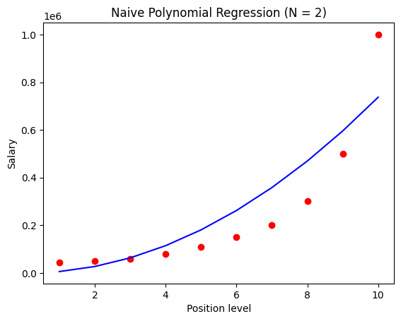
We use the entire dataset for better visualization because only test dataset won’t give a clear idea because the size of our dataset is too small. Using the complete dataset will enable us to get a better insight.

We use the entire dataset for all the visualizations ahead in the notebook too.

pred_plot = pred_to_plot(W_trained,X)

plt.scatter(X[:,0], y, color = 'red')
plt.plot(X[:,0], pred_plot, color = 'blue')
plt.title('Naive Polynomial Regression (N = 2)')
plt.xlabel('Position level')
plt.ylabel('Salary')
plt.show()

We have got good results for \(N=2\) but we can try for better performance by changing the value of \(N\).

Let us train the regressor for \(N=4\).

8.2.6. Polynomial Regression (N=4)

# Independent Feature
X = np.asarray(dataset['Level'].values.tolist())

# Reshaping the independent feature
X = X.reshape(-1,1)

# Constructing the polynomials of our Independent features 
X_poly = poly_features(4,X)

C:\Users\Administrator\AppData\Local\Temp\ipykernel_2680\424119940.py:21: FutureWarning: In a future version, `df.iloc[:, i] = newvals` will attempt to set the values inplace instead of always setting a new array. To retain the old behavior, use either `df[df.columns[i]] = newvals` or, if columns are non-unique, `df.isetitem(i, newvals)`
  data.iloc[:,i-1] = (X**i).reshape(-1,1)

array([[ 1],
       [ 2],
       [ 3],
       [ 4],
       [ 5],
       [ 6],
       [ 7],
       [ 8],
       [ 9],
       [10]])

#Adding the feature X0 = 1, so we have the equation: y =  W0 + (W1 * X1) + (W2 * (X1**2))
X_poly = np.concatenate((___,___.___((___,___))), axis = 1)

X_poly

array([[1.000e+00, 1.000e+00, 1.000e+00, 1.000e+00, 1.000e+00],
       [2.000e+00, 4.000e+00, 8.000e+00, 1.600e+01, 1.000e+00],
       [3.000e+00, 9.000e+00, 2.700e+01, 8.100e+01, 1.000e+00],
       [4.000e+00, 1.600e+01, 6.400e+01, 2.560e+02, 1.000e+00],
       [5.000e+00, 2.500e+01, 1.250e+02, 6.250e+02, 1.000e+00],
       [6.000e+00, 3.600e+01, 2.160e+02, 1.296e+03, 1.000e+00],
       [7.000e+00, 4.900e+01, 3.430e+02, 2.401e+03, 1.000e+00],
       [8.000e+00, 6.400e+01, 5.120e+02, 4.096e+03, 1.000e+00],
       [9.000e+00, 8.100e+01, 7.290e+02, 6.561e+03, 1.000e+00],
       [1.000e+01, 1.000e+02, 1.000e+03, 1.000e+04, 1.000e+00]])

y

array([[  45000],
       [  50000],
       [  60000],
       [  80000],
       [ 110000],
       [ 150000],
       [ 200000],
       [ 300000],
       [ 500000],
       [1000000]])

#Splitting the dataset
X_train, y_train, X_test, y_test = split_data(X_poly,y)

#declaring the "regressor" as an object of the class LinearRegression
regressor = polynomialRegression()

#Training 
W_trained, train_loss, num_epochs = regressor.train(X_train, y_train, epochs=1000, alpha=1e-9)

#Testing on the Test Dataset
test_pred, test_loss = regressor.test(X_test, y_test, W_trained)

X_poly

array([[1.000e+00, 1.000e+00, 1.000e+00, 1.000e+00, 1.000e+00],
       [2.000e+00, 4.000e+00, 8.000e+00, 1.600e+01, 1.000e+00],
       [3.000e+00, 9.000e+00, 2.700e+01, 8.100e+01, 1.000e+00],
       [4.000e+00, 1.600e+01, 6.400e+01, 2.560e+02, 1.000e+00],
       [5.000e+00, 2.500e+01, 1.250e+02, 6.250e+02, 1.000e+00],
       [6.000e+00, 3.600e+01, 2.160e+02, 1.296e+03, 1.000e+00],
       [7.000e+00, 4.900e+01, 3.430e+02, 2.401e+03, 1.000e+00],
       [8.000e+00, 6.400e+01, 5.120e+02, 4.096e+03, 1.000e+00],
       [9.000e+00, 8.100e+01, 7.290e+02, 6.561e+03, 1.000e+00],
       [1.000e+01, 1.000e+02, 1.000e+03, 1.000e+04, 1.000e+00]])

8.2.6.1. Visualizing Results

pred_plot = pred_to_plot(W_trained,X_poly)

pred_plot

[101.56686988148302,
 1570.332736753576,
 7876.252690310476,
 24783.645533405484,
 60351.39230382515,
 124932.93627428928,
 231176.28295245094,
 394024.0000808964,
 630713.2176371454,
 960775.6278336504]

plt.scatter(X_poly[:,0], y, color = 'red')
plt.plot(X_poly[:,0], pred_plot, color = 'blue')
plt.title('Naive Polynomial Regression (N=4)')
plt.xlabel('Position level')
plt.ylabel('Salary')
plt.show()

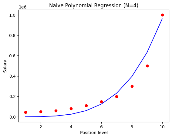
Clearly, the regressor with \(N=4\) performs better than the regressor with \(N=2\). You can increase the value of \(N\) and look for better performance but, be careful that you don’t run into the problem of Overfitting.

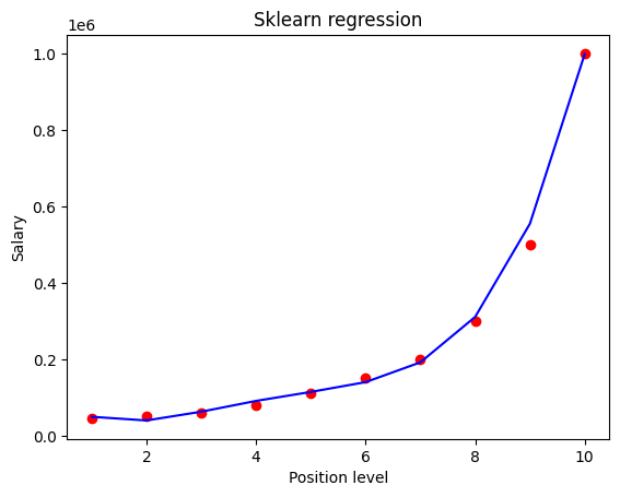
As of now, our best regressor has \(N=4\) and therefore, we will train the polynomial regression using sklearn only for \(N=4\)

8.3. Polynomial Regression using Sklearn

8.3.1. Importing dependencies

import numpy as np
import pandas
import matplotlib.pyplot as plt 
from sklearn.model_selection import train_test_split
from sklearn.linear_model import LinearRegression
from sklearn.preprocessing import PolynomialFeatures

8.3.2. Data Preprocessing

#Get the Dataset and separating the independent and dependent features
dataset = pd.read_csv(r'../../dataset/Position_Salaries.csv')
X_sk = dataset.iloc[:, 1].values
y_sk = dataset.iloc[:, -1].values

#Reshaping the Independent amd Dependent Features
X_sk = X_sk.reshape(-1,1)
y_sk = y_sk.reshape(-1,1)

# Constructing the polynomials of our Independent features 
poly_reg = PolynomialFeatures(degree = 4)
X_poly_sk = poly_reg.fit_transform(X_sk)

#Get the shapes of X and y
print("The shape of the independent fatures are ",X_poly_sk.shape)
print("The shape of the dependent fatures are ",y_sk.shape)

The shape of the independent fatures are  (10, 5)
The shape of the dependent fatures are  (10, 1)

X_poly_sk

array([[1.000e+00, 1.000e+00, 1.000e+00, 1.000e+00, 1.000e+00],
       [1.000e+00, 2.000e+00, 4.000e+00, 8.000e+00, 1.600e+01],
       [1.000e+00, 3.000e+00, 9.000e+00, 2.700e+01, 8.100e+01],
       [1.000e+00, 4.000e+00, 1.600e+01, 6.400e+01, 2.560e+02],
       [1.000e+00, 5.000e+00, 2.500e+01, 1.250e+02, 6.250e+02],
       [1.000e+00, 6.000e+00, 3.600e+01, 2.160e+02, 1.296e+03],
       [1.000e+00, 7.000e+00, 4.900e+01, 3.430e+02, 2.401e+03],
       [1.000e+00, 8.000e+00, 6.400e+01, 5.120e+02, 4.096e+03],
       [1.000e+00, 9.000e+00, 8.100e+01, 7.290e+02, 6.561e+03],
       [1.000e+00, 1.000e+01, 1.000e+02, 1.000e+03, 1.000e+04]])

8.3.3. Polynomial Regression

# Splitting the dataset into the Training set and Test set
X_train_sk, X_test_sk, y_train_sk, y_test_sk = train_test_split(X_poly_sk, y_sk, test_size = 0.2, random_state = 0)

# Fitting Simple Linear Regression to the Training set
regressor_sk = LinearRegression()
regressor_sk.fit(X_train_sk, y_train_sk)

LinearRegression()

In a Jupyter environment, please rerun this cell to show the HTML representation or trust the notebook.
On GitHub, the HTML representation is unable to render, please try loading this page with nbviewer.org.

8.3.3.1. Visualizing the results

plt.scatter(X_poly_sk[:,1], y, color = 'red')
plt.plot(X_poly_sk[:,1], regressor_sk.predict(X_poly_sk), color = 'blue')
plt.title('Sklearn regression')
plt.xlabel('Position level')
plt.ylabel('Salary')
plt.show()

8.4. Acknowledgments

Thanks to Jay Pradip Shah for creating the open-source course Polynomial Regression from scratch. It inspires the majority of the content in this chapter.